17 KiB
Big O Cheatsheet
This is just a cheat sheet containing some observations about common for loop patterns taken from Abdul Bari's video series on algorithms.
For Loops
\mathcal{O}(n) for (i = 0; i < n; i++) {} // \mathcal{O}(n)
for (i = 0; i < n; i = i + 2) {} // = n/2 = \mathcal{O}(n)
for (i = n; i > 1; i--) {} // \mathcal{O}(n)
\mathcal{O}(n^2) for (i = 0; i < n; i++) {
for (j = 0; j < n; j++) {} // \mathcal{O}(n^2)
}
\mathcal{O}(log_2(n)log_2(p)) for (i = 1; i < n; i = i * 2) {
p++; // log_2(n)
}
for (j = 1; j < p; j = j * 2) {
// log_2(p)
}
// log_2(n) + log_2(p) = \mathcal{O}(log_2(n)log_2(p))
\mathcal{O}(log_2(n)) for (i = 1; i < n; i = i * 2) {} // \mathcal{O}(log_2(n))
for (i = n; i > 1; i = i / 2) {} // \mathcal{O}(log_2(n))
\mathcal{O}(log_3(n)) for (i = 1; i < n; i = i * 3) {} // \mathcal{O}(log_3(n)
While Loops
\mathcal{O}(n) i = 0;
while (i < n) {
i++;
} // \mathcal{O}(n)
\mathcal{O}(log_2(n)) a = 1;
while (a < b) {
a = a * 2;
} // \mathcal{O}(log_2(n))
/* NOTE:
a >= b
a = 2^k // where k represents unknown value of b
2^k >= b // condition where loop stops
2^k = b // by making condition where loop stops true...
k = log_2(b) we can determine that unknown value b stops when k is equal to log_2 of b
which evaluates to: \mathcal{O}(log_2(n))
*/
i = n;
while (i > 1) {
    i = i / 2;
}
\mathcal{O}(\sqrt n) i = 1;
k = 1;
while (k < n) {
k = k + i;
i++;
}
Analyzing the above with some dummy data:
| i | k |
|---|---|
| 1 | 1 |
| 2 | 1 + 1 |
| 3 | 2 + 2 |
| 4 | 2 + 2 + 3 |
| 5 | 2 + 2 + 3 + 4 |
| m | ...m |
Which in mathematical notation would be:
\frac{m(m + 1)}{2} We can further analyze this like so:
k \geq n \frac{m(m + 1)}{2} \geq n m^2 \geq n m = \sqrt n Thusly the big O notation of this is:
\mathcal{O}(\sqrt n) Note that this is not the same as log_2(n). For an explanation of this, please see this stack overflow answer. According to other sources (GPT), the time complexity of
\mathcal{O}(\sqrt n) is often unavoidable when a matrix of values is unsorted.
While loops with If Statements
\mathcal{O}(n) The following demonstrates evaluating the GCD(Greatest Common Divisor) between two numbers:
while (m != n)
{
    if (m > n)
        m = m - n;
    else
        n = n - m;
}
Let's take a look at an example where both m and n start off as equal:
| m | n |
|---|---|
| 5 | 5 |
Since they are equal the condition:
while (m != n)
Will never execute, thus the amount of execution steps is 0. Let's look at another example:
| m | n |
|---|---|
| 14 | 2 |
In this case, the condition:
if (m > n)
    m = m - n;
Evaluates to true and the value of m is equal to m - n, replaced with `14
- 2
, and thuslymis equal to12`. This continually evaluates down the line like so:
| m | n |
|---|---|
| 14 | 2 |
| 12 | 2 |
| 10 | 2 |
| 8 | 2 |
| 6 | 2 |
| 4 | 2 |
| 2 | 2 |
At which point the loop stops because the condition:
while (m != n)
Evaluates to false, and the loop ends, resulting in the loop having executed 7
times. We add 1 to the amount of times it is executed by nature of the initial
loop, and it is 8. This evaluates to
\frac{16}{2} or:
\frac{n}{2} Which, in big O notation, evaluates to:
\mathcal{O}(n) The minimum time to execute is at least one time, thusly the minimum time complexity is:
\mathcal{O}(1) Best Case vs. Worst Case
void some_algo_test(int n)
{
    if (n < 5)
        printf("%d\n", n); // 1
    else
        for (int i = 0; i < n; i++)
            printf("%d\n", i); // n
}
This evaluates in best case to:
\mathcal{O}(1) This happens when the condition n < 5 evaluates to true, because all it does
is print the value of n to the console.
Otherwise, if n < 5 evaluates to false (i.e. n is a value greater than or
equal to 5), then the worst case time complexity occurs, which is:
\mathcal{O}(n) In essence:
BEST CASE:
\mathcal{O}(1) WORST CASE:
\mathcal{O}(n) Now let's adjust our function a bit:
void some_algo_test(int n)
{
    if (n < 5)
        printf("%d\n", n); // 1
    for (int i = 0; i < n; i++)
        printf("%d\n", i); // n
}
Note here, that now, the for loop executes regardless of the if (n < 5)
condition. Thusly the best and worst case scenario become the same:
\mathcal{O}(n) Types of Time Functions
Constant:
\mathcal{O}(1) Logirithmic:
\mathcal{O}(log(n)) Square Root:
\mathcal{O}(\sqrt n) Linear:
\mathcal{O}(n) Linearithmic:
\mathcal{O}(n(log(n))) Quadratic:
\mathcal{O}(n^2) Cubic:
\mathcal{O}(n^3) Exponential:
\mathcal{O}(2^n) Order of Types of Time Function
1 < log(n) < \sqrt n < n < n(log(n)) < n^2 < n^3 < ... 2^n < 3^n .... < n^n 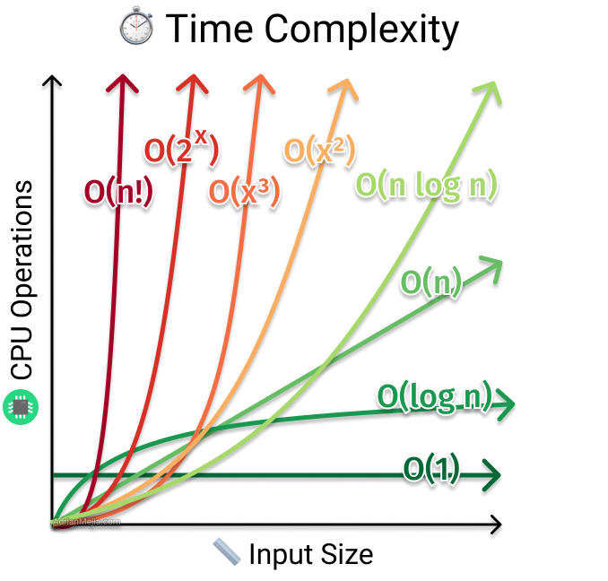
Asymptotic Notation
There are generally three types of Asymptotic Notation, which is a type of Mathematical Notation to denote time/space complexity of a particular algorithm.
There is what is known as "Big O" (pronounced "big-oh") notation:
\mathcal{O} Which represents the Upper Bound.
There is "Big-Omega":
\Omega Which represents the Lower Bound.
And there is also "Theta":
\Theta Which represents the Average Bound.
Big O In Mathematical Notation
Big O Notation:
\mathcal{O}(n) Big O is the most common notation utilized in computer science for representing the Upper Bound or Worst Case Time Complexity of an algorithm. Let us take a look at how Linear Time Complexity is represented in mathematical notation:
f(n) = \mathcal{O}(g(n)) \iff \exists +ve\ constant\ c\ and\ n_0 Which generally means that the function f takes the argument n, which equals
the \mathcal{O} of positive numbers c and n0 if and only if c and n_0
exist.
The inequality condition reads as follows:
\mid f(n) \leq c * g(n) \forall n \geq n_0 Which generally means such that f(n) is greater than or equal to c into
g(n) for all that n are greater than or equal to n_0.
This culminates in the final mathematical notationof:
f(n) = \mathcal{O}(g(n)) \iff \exists +ve\ constant\ c\ and\ n_0 \mid f(n) \leq c * g(n) \forall n \geq n_0 Demonstration:
Let's fill in our variables other than n to demonstrate:
f(n) = 2n + 3 If we follow this by filling in a condition where this function is true like so:
2n + 3 \leq 10n Where the number 10 fills in for the variable c, and the expression 2n + 3
stands in for our function, f(n).
This will be true as long as n is greater than or equal to 1, thusly, we can
further express this as:
\forall n \geq 1,\ 2n + 3 \leq 10n Which, again, basically means 2n + 3 is less than or equal to 10n for all
cases where n is greater than or equal to 1.
While accurately depicting the actual time complexity of our algorithm, Asymptotic Notation is meant to be the most general form of notation to communicate what our worst time or space complexity is, thusly, we can narrow this down to:
f(n) \leq c * g(n) Which can be further generalized as simply:
f(n) = \mathcal{O}(n) \mathcal{O}(n^2) Quadratic Time Complexity can be expressed very similarly with a demonstration like so:
Let's fill in our variables slightly differently:
2n + 3 \leq 2n^2 + 3n^2 Which would evaluate to:
2n +3 \leq 5n^2 This would be true for all conditions where the value of n is greater than or
equal to 1. We can express this like so:
\forall n\geq 1,\ 2n+3 \leq 5n^2 This is further simplified as the following expression:
f(n) \leq c * g(n^2) Or, very simply, and at our final Big O notation:
f(n) = \mathcal{O}(n^2) Classifications of Bounds
Linear Time Complexity is generally considered "Average Bound", while Constant Time, Logirithmic Time, and Square Root Time Complexities are considered "Lower Bound". All other Time Complexities Are considered "Upper Bound" Time Complexity Classifications
Let us now look at the lower bound notation, Big Omega:
Big Omega Notation:
\Omega The mathematical notation that defines Big Omega reads as follows:
f(n) = \Omega(g(n)) \iff \exists +ve\ constant\ c\ and\ n_0 Which essentially means "the function f(n) is equal to 'Omega', \Omega, of
g(n) if and only if there exists postiive constants c and $n_0$".
And the conditional reads as follows:
\mid f(n) \geq c * g(n) \forall n \geq n_0 Which essentially means such that "such that the function f(n) is greater than
or equal to c into g(n) for all cases where n is greater than or equal to
$n_0$"
Demonstration:
If we fill in our variables, we can demonstrate how to further deduce Big Omega Notation:
Let us take the case where f(n) is equal to the mathematical expression
2n+3:
f(n) = 2n + 3 We can further express this as:
2n + 3 \geq 1n Of course, this condition only is true for all cases where n is greater than
or equal to 1, so we must express that as:
\forall n \geq 1, 2n + 3 \geq 1n This, simplifies to:
f(n) = \Omega(n) Of course, if we change expression:
2n + 3 \geq 1n To:
2n + 3 \geq 1(log(n)) This would also be a true expression for our function f(n). This would be
expressed as:
f(n) = \Omega(log(n)) Because \Omega represents the time complexity that is within the "Lower
Bound", or our "Best Case Scenario Time/Space Complexity", only time
complexities within \mathcal{O}(1), \mathcal{O}(log(n)), and
\mathcal{O}(\sqrt n) are considered to be able to be represented by \Omega
because they fall within the lower bound. Thusly Big Theta or Big O notations
larger than \mathcal{O}(\sqrt n) are not represented within \Omega notation.
This nearly wraps up our notations, all that's left is Theta Notation.
Big Theta Notation:
\Theta The mathematical notation that defines Big Theta reads as follows:
f(n) = \Theta(g(n)) \iff \exists +ve\ constant\ c_1\, c_2\ and\ n_0 Which essentially means "the function f(n) is equal to 'Theta', \Theta, of
g(n) if and only if there exists postiive constants c_1, c_2, and $n_0$".
And the conditional reads as follows:
\mid c_1 * g(n) \leq f(n) \leq c_2 * g(n) Which essentially means such that "such that the value of c_1 into g(n) is
less than or equal to the output of the function f(n), which itself must also
be less than or equal to the value of c_2 into g(n).
Demonstration:
We can demonstrate Theta notation with the following example. Consider the following function expression:
f(n) = 2n + 3 This can be further expressed by defining a lower and upper bound in which our function expression exists:
1n \leq 2n + 3 \leq 5n Note here how we are filling in our variables. In this case, c_1 is 1,
g(n) is n, our function f(n) is 2n + 3, c_2 is 5, and again, g(n)
is n. We are "constraining" our function f(n), saying that in order for it
to be represented by \Theta notation, the return value of f(n) must exist
between these two conditional statements(i.e. 1n \leq and \leq 5n).
This expression can be further simplified as:
f(n) = \Theta(n) Note that this expression is the only expression allowed by \Theta notation.
This is because it lives within the "Average" bound.
NOTE: It is important to note that oftentimes Developers/Mathematicians
conflate these notations with "Best Case" or "Worst Case" time/space
complexities. This is incorrect. These are simply classifications under which
these notations usually fall when conveying the efficiency of an algorithm. All
three forms of notation, \mathcal{O}, \Omega, and \Theta can be used to
express "Best", and "Worst" case time/space complexities, which will be covered
in a future section.
Further Examples:
All Three Notations:
Let's take this function, which, as you'll eventually see, can be expressed in
all three forms of notation (\mathcal{O}, \Omega, and \Theta):
f(n) = 2n^2 + 3n + 4 We can express this as:
2n^2 + 3n + 4 \leq 2n^2 + 3n^2 + 4n^2 Which is further simplified as:
2n^2 + 3n + 4 \leq 9n^2 Where 9 represents in our classical expression of previous notations as c
and n^2 represents g(n). Thusly, we can take the value of g(n) in this
case and plug it into our final expression:
f(n) = \mathcal{O}(n^2) If we take the same function:
f(n) = 2n^2 + 3n + 4 And then say that it must always be greater than or equal to 1*n^2:
2n^2 + 3n + 4 \geq 1n^2 This evaluates based off of our previous notations to be represented in \Omega
notation like so:
\Omega(n^2) If we then further restrict our condition as:
1n^2 \leq 2n^2 + 3n + 4 \leq 9n^2 Can be represented as:
\Theta(n^2) To reiterate, the representation of g(n) in our formulas takes the place of
our time/space complexity notation. Let's take another example to reiterate
this:
f(n) = n^2(log(n)) + n Can be evaluated with the condition:
1n^2(log(n)) \leq n^2(log(n)) + n \leq 10n^2(log(n)) Because the first expression:
1n^2(log(n)) \leq n^2(log(n)) Fulfills the condition for \Omega notation due to the condition required by
\Omega:
\mid f(n) \geq c * g(n) \forall n \geq n_0 We can say that the following notation:
\Omega(n^2(log(n))) Is true.
Additionally, the expression:
n^2(log(n)) + n \leq 10n^2(log(n)) Fulfills the condition for \mathcal{O}) notation due to the condition required
by \mathcal{O}:
\mid f(n) \leq c * g(n) \forall n \geq n_0 We can say that the following notation:
\Omega(n^2(log(n))) Also is true.
And also, we find that because the expression:
1n^2(log(n)) \leq n^2(log(n)) + n \leq 10n^2(log(n)) Also fulfilles \Theta notation's constraints by being restricted between a
lower and upper bound that fulfills $\Theta$'s conditional:
\mid c_1 * g(n) \leq f(n) \leq c_2 * g(n) We can also say that this is true:
\Theta(n^2(log(n)))Thusly our function can be truthfully expressed in all three notations:
\mathcal{O}(n^2(log(n))) \Omega(n^2(log(n))) \Theta(n^2(log(n))) Only Two Notations:
Let's say we have a function that simply returns a factorial of the variable
n:
f(n) = n! As a refresher, this can be expressed as so:
f(n) = n! = n * (n - 1) * (n - 2) * ... 3 * 2 * 1 We can further express its bounds like so:
1 * 1 * 1 * 1... *1 \leq 1 * 2 * 3 ... * n \leq n * n * n * n * n * n ... * n Because this evaluates to:
1 \leq n! \leq n^n We can see that there is no g(n) defined on our lower bound, and thusly it
does not fulfill the condition required by \Theta notation. As a reminder that
condition is:
\mid c_1 * g(n) \leq f(n) \leq c_2 * g(n) Thusly we can only express this in \mathcal{O} and \Omega notation:
\mathcal{O}(n^n) \Omega(1) This is because in order for the "Average" bound to be calculated, it would have
to calculate all values of n! between 1 and n!, and thusly any attempt to
express the time/space complexity of f(n) would not have little use when
compared with other notations. To hammer it home, consider that this statement
cannot always be true:
n^10 < n! < n^11 This cannot always be true, and if we cannot find a "middle" or
"average" bound, then we cannot express our time/space complexity in \Theta
notation.
Expressing log(n) factorial
Suppose I have the following mathematical expression:
f(n) = log(n!) This is equivalent to:
log(1 * 2 * 3... * n) We can express a true conditional that:
log(1 * 1 * 1 * 1 ... * 1) \leq log(1 * 2 * 3 ... * n) \leq log(n * n * n ... * n) This simplifies in expression down to:
1 \leq log(n!) \leq log(n^n) Which is further simplified as:
1 \leq log(n!) \leq n(log(n)) Once again, we have found that we cannot express an "Average bound" within this conditional. Thusly we can express our time/space complexity as follows:
\mathcal{O}(n(log(n))) and:
\Omega(1) Again, this can be proven to have no discernable "Average" bound like so:
log(1) < 1! < 1^11 Which is not true.